Building Netron OCR: Four Models, One Screenshot
How I turned photographed Netron graphs into editable JSON with four compact vision models, a synthetic camera simulator, and a hand-annotated real-world evaluation set.
I started Netron OCR with an apparently direct plan: give a model a screenshot of an ONNX graph open in Netron and ask it to emit the graph as JSON.
The idea grew out of experiments with multimodal LLMs. They could follow the overall graph, yet routinely missed small tensor shapes, merged nearby nodes, or invented connections. When I supplied the same model with a precise textual graph description, reconstruction became much more reliable, which pointed to a dedicated visual front end for translating Netron pixels into structured data.
My first end-to-end OCR experiments attempted that entire translation at once: locate nodes, identify operators, read labels, preserve order, and produce valid JSON. Much of the model’s capacity went into braces, commas, and sequence alignment before it could read the graph reliably, and the best early node-only token model produced valid JSON just 12.6% of the time, with a node F1 of 2.9%.
Those results led me to divide the visual work into four tasks, each operating at the scale and output space suited to its target.
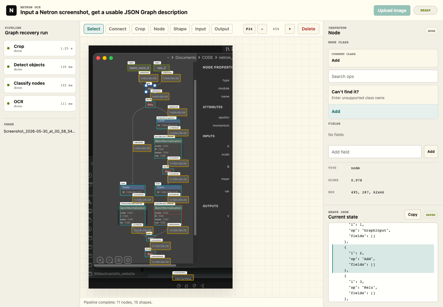
The current workbench keeps the source image, editable detections, node inspector, and graph JSON in one place. The models do the repetitive visual work; the user can correct the remaining ambiguity.
1. One image, four specialists
The deployed pipeline contains roughly 6.7M parameters across four models, with a defined job, input scale, and evaluation metric for every stage.
| Stage | Job | Architecture |
|---|---|---|
| Cropper | Isolate the useful Netron canvas from a full screenshot or phone photo | 405K-parameter depthwise CNN with horizontal and vertical projection heads |
| Detector | Find nodes, tensor-shape labels, graph inputs, and graph outputs | 2.35M-parameter anchor-free Tiny-YOLO with a stride-4 feature pyramid |
| Classifier | Assign one of 72 ONNX operator classes to each detected node | 2.71M-parameter depthwise CNN over 160×96 node crops |
| OCR | Transcribe variable tensor-shape strings such as 1×64×56×56 | 1.26M-parameter patch encoder with a Transformer and cross-attentive GRU decoder |
I trained each model independently on a single GPU and selected checkpoints using synthetic validation data, reserving the real photographs for report-only evaluation.
1.1 The cropper: lose background, never lose a node
A phone photo of Netron captures several nested scenes: the desk, the screen, the application window, and finally the graph. Browser toolbars, wallpaper, side panels, keyboards, and even the photographer’s reflection all become part of the input.
The cropper sees a 512×512 version of the full image. A direct four-coordinate regressor seemed natural, although a slightly tight box can remove an input pill or the final tensor label and damage every downstream stage. I chose a depthwise CNN that predicts horizontal and vertical content projections over 128 bins; those projections define the occupied region, and a second head learns a safe margin for each edge.
The training objective therefore assigns a higher cost to clipping graph content than to retaining a little extra background. On the 74-image real evaluation set, the selected cropper retained every manually annotated node, tensor shape, input, and output with zero missed important area, even before the deployed 4% safety padding.
1.2 The detector: keep the small text alive
After cropping, one shared detector locates four visual classes: nodes, graph inputs, graph outputs, and tensor-shape labels. Tensor strings make the last class especially difficult because they are tiny, numerous, and visually closer to ordinary interface text than to a node card.
To keep deployment lightweight, I built a compact, framework-independent Tiny-YOLO whose depthwise backbone feeds a feature pyramid. At 320×384, its stride-4 head predicts anchor-free center heatmaps and box dimensions, preserving the small tensor labels that would disappear with more aggressive downsampling.
Rare graph I/O objects and small tensor labels receive class-aware sampling and loss weights. The resulting detector has about 2.35M parameters and reached 0.869 mean box F1 across the four classes on the manual real-image set.
1.3 The classifier: use the closed vocabulary
Because node titles come from a vocabulary of 72 common ONNX operators, I treated their recognition as classification. Limiting the prediction to those known classes removes the many possible misspellings of BatchNormalization and lets the network concentrate on the visual differences between operator cards.
The node classifier is a four-stage depthwise CNN with global pooling and a small MLP head. Detector boxes are projected back into the source-image coordinate system before the 160×96 patches are extracted, allowing the recognizer to use high-resolution source pixels after a fast, low-resolution detection pass.
Training crops are intentionally imperfect: padding varies from 0 to 14 pixels, boxes receive small geometric jitter, and color, contrast, blur, and noise change from sample to sample. This variation stopped the classifier from assuming that every operator card would be centered, tightly cropped, and rendered in the same theme.
1.4 The OCR model: reserve sequence decoding for sequences
Tensor-shape values vary from graph to graph, which calls for character-level OCR. The model reads 160×48 crops as 8×8 visual patches, builds their image representation with two Transformer encoder layers, and uses a two-layer autoregressive GRU with cross-attention to decode up to 32 characters. At 1.26M parameters, it runs comfortably inside an interactive pipeline while still resolving small differences between strings such as 1×8×56×56 and 1×8×56×55.
Confining sequence decoding to variable tensor text reduced both the computational cost and the error surface of operator recognition, making this division of work one of the most consequential architecture decisions in the project.
2. Building a camera into the dataset
Model design covered only part of the project, because training the pipeline required more labeled phone photos of Netron graphs than were available. I therefore generated the dataset myself.
The generator creates valid ONNX models from a 72-operation vocabulary, runs shape inference, opens each model in the real Netron application, and captures the visible graph through a browser. Since the source graph already provides the nodes, tensor shapes, inputs, outputs, and graph structure, every screenshot arrives with exact metadata generated alongside it.
The final audited dataset contains 53,824 rendered scenes and about 1.1M visual boxes. From the same source corpus I derived detector examples, more than 223K node-classification patches, and hundreds of thousands of tensor-shape crops.
The first real photos exposed how far my clean, centered renders were from a camera image. Perspective, large reflections, uneven lighting, screen moiré, tiny zoomed-out graphs, browser chrome, and unrelated text all widened the synthetic-to-real gap.
To close that gap, the data pipeline grew into a camera simulator. It adds perspective and rotation, exposure gradients, white-balance shifts, radial glare, reflection-like light bands, shadows, vignetting, moiré, chromatic fringing, resizing blur, JPEG artifacts, and sensor-like noise. It also embeds the Netron window over varied wallpaper and software backgrounds, at different scales and aspect ratios, with synthetic window chrome and visual distractors around it.
Several early augmentation previews became unreadable even to me because blur-like effects could accumulate without limits. I stopped those runs and capped their combined strength, keeping the simulated artifacts varied while preserving the graph information a person could reasonably recover from a photograph.
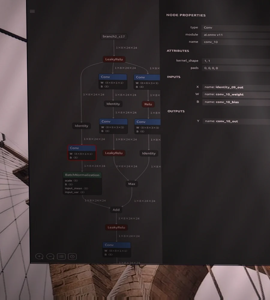
A generated training scene: a real Netron render placed inside an unrelated desktop background, then transformed by the camera simulator.
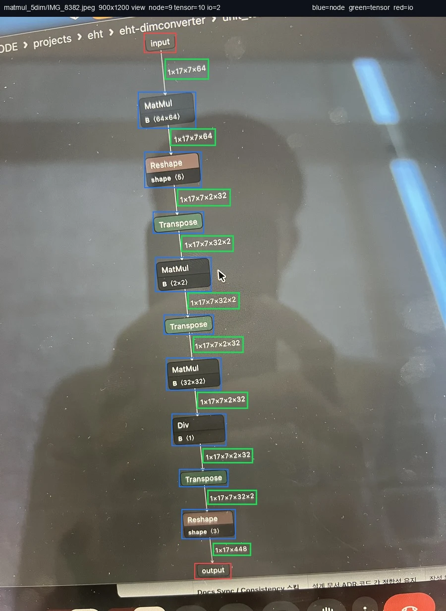
A hand-annotated real photo. Blue boxes mark nodes, green boxes mark tensor shapes, and red boxes mark graph I/O. The benchmark keeps the reflection exactly as photographed.
3. A benchmark made by hand
Synthetic validation measures how well each network learned the generated tasks, while transfer to real screens requires separate evidence. I created that evidence by taking 74 screenshots and phone photos of 14 different ONNX graphs, then manually annotated 663 nodes, 807 tensor-shape labels, and 129 graph inputs and outputs: 1,599 boxes in total.
The entire set stayed outside training, checkpoint selection, threshold selection, and hyperparameter tuning, serving only as a report card for the finished stages. This separation prevented the benchmark from quietly becoming training data through repeated decisions, even when its results made a promising synthetic improvement look less impressive.
Because the stages use different evaluation sources, each metric carries its own scope:
- The cropper’s
100%containment and the detector’s0.869mean box F1 come from the 74-image manual set. - The node classifier reached
99.85%accuracy on a held-out synthetic test set. - Tensor-shape OCR reached
96.68%exact match and99.19%character accuracy on8,192held-out synthetic crops.
The classifier and OCR figures measure held-out synthetic data, with real-image galleries serving as qualitative diagnostics for those stages. Keeping the evaluation scope beside each number avoids combining four differently measured results into a misleading end-to-end score.
4. Why I kept the editor
The four learned stages now recover the Netron canvas, visual objects, operator classes, and tensor text. Connections can remain visually ambiguous in a photograph, so the current prediction payload deliberately leaves topology open; the workbench then lets the user draw or correct edges, attach nearby tensor shapes, edit fields, and inspect the JSON as it changes.
That human-in-the-loop boundary reflects the cost of a wrong edge, which can change the meaning of the model. A quick correction resolves the remaining ambiguity, and the resulting graph description gives an LLM the structured input it needs to rebuild an ONNX model reliably.
You can try the live Netron OCR demo or read the shorter project overview.
Building the system this way gave every failure a clear location: cropping, localization, operator recognition, or transcription. A tight crop, missed box, confused operator, or wrong character now appears in a stage with its own metric and visual output to inspect. With the earlier screenshot-to-JSON model, all of those faults surfaced as one malformed string; in the four-stage pipeline, each became an engineering problem I could measure and improve.